Money Supply & Other Inflation Factors

Overview

Milton Friedman founded modern monetarism on the first principal assumption that, “inflation is always and everywhere a monetary phenomenon.” Monetarism remained the preeminent economic theory from the 1960’s through the 1990’s, with growth in the money supply (M2, a measure of the money supply including all physical cash and checking deposits plus “near money,” such as savings deposits, money market securities, and other time deposits that can be quickly converted into cash) correlated with subsequent inflation roughly two years later (but with variable lags). The relationship between money supply and inflation started to breakdown around the year 2000. M2 expanded steadily through the 2000s and surged during the quantitative easing programs of the 2010s, yet consumer price inflation remained stubbornly low. Many economists concluded that monetarism was obsolete—a relic of the Reagan/Volcker era (see document link below for more information about this interesting chapter in US economic history). The Covid-19 pandemic may have reasserted monetarist theory, as M2 surged 24.7% in 2020, the largest single-year expansion in modern history, and CPI peaked at 8.0% two years later in 2022—almost exactly on schedule. It is essentially impossible to isolate and identify any linear relationship between distinct inflation-related variables (in this case M2 and CPI) because there are so many factors at play on inflation at any given time. Globalization, technology enabled efficiency and productivity gains, and favorable demographics and deregulation all served to offset monetary led inflation in the first two decades of the 2000’s leading to the illusion that inflation was no longer “always” a monetary phenomenon.

Money Supply Growth Leads Inflation by ~2 Years

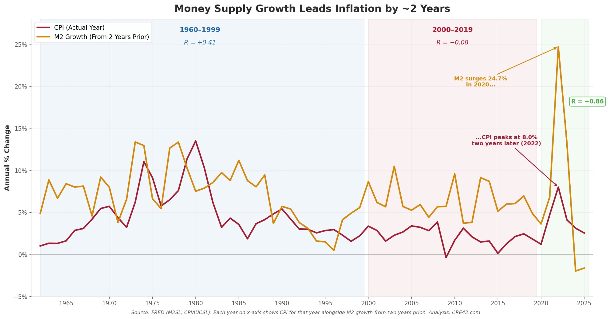
M2 Growth vs. CPI with 2-Year Lag, 1962–2025

M2 annual growth rate (shifted forward two years) overlaid with CPI annual change, 1962–2025. Era shading reflects distinct correlation regimes. Source: FRED (M2SL, CPIAUCSL). Analysis: CRE42.com

Document Links

inflation-money-supply.xlsx — M2 and CPI annual data (1960–2025), 2-year lag analysis, era and decade correlations, embedded charts, methodology

Key Takeaways

Three Distinct Eras of Money–Inflation Correlation From 1960–1999, M2 growth correlated with CPI two years later with a correlation (R) of R = +0.41. From 2000–2019, that correlation collapsed to R = −0.08 as powerful disinflationary forces absorbed monetary expansion. From 2020–present, the relationship reasserted at R = +0.86—the strongest reading across all three eras.

The ~24-Month Lag Is Structural, Not Coincidental New money flows through a transmission chain: financial assets and bank reserves first (months 0–6), business pricing and wage negotiations next (months 6–18), and finally CPI—especially the shelter component, which accounts for one-third of the index and lags actual market rents by 12–18 months. Friedman himself cited “long and variable lags” peaking near 18–24 months, consistent with Federal Reserve and BIS research.

2000–2019 The post-millennial money supply/inflation relationship breakdown was likely not a failure of monetary theory but a consequence of extraordinary countervailing forces: globalization suppressed goods prices, labor supply was high with baby boomers in their prime work years (arguably influencing in turn the weakening of labor unions), technology deflated information and logistics costs, and deregulation reduced friction and prices across the economy.

The Forward Question: Are Disinflationary Forces Reasserting or Reversing? M2 contracted in 2022–2023 for the first time since the 1930s, which the two-year lag framework would predict as disinflationary in 2024–2025. However, several of the forces that suppressed inflation during 2000–2019—globalization, demographic tailwinds, and low energy costs—are now partially reversing, while AI-driven productivity gains represent a potentially powerful new disinflationary force. The net direction of these competing pressures is one of the defining investment questions of the next decade.

2-Year Lag Correlation by Decade

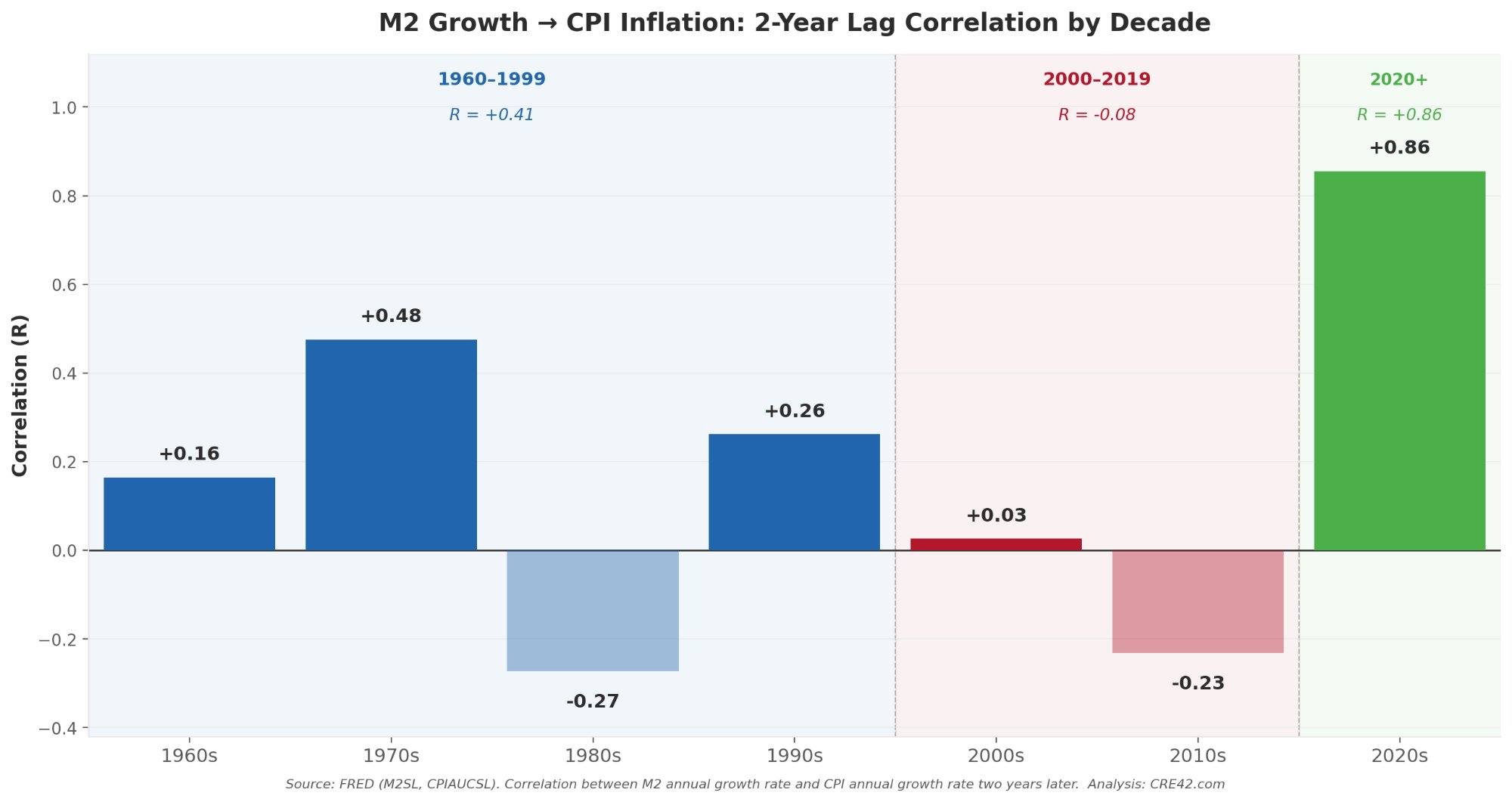
Correlation (R) between M2 annual growth rate and CPI annual change two years later, by decade. Color shading matches the three-era framework. Source: FRED (M2SL, CPIAUCSL). Analysis: CRE42.com

Three Eras of Money & Inflation

1960–1999: Money Supply Growth Correlated with Inflation

For four decades, the relationship between money supply growth and subsequent inflation was visible and broadly consistent. The 1970s provided the most dramatic confirmation—rapid M2 expansion fueled by deficit spending, oil shocks, and accommodative monetary policy produced the highest peacetime inflation in American history, with CPI regularly exceeding 10%. The decade produced a 2-year lag correlation of R = +0.48, the strongest of the pre-2000 era. Paul Volcker’s aggressive rate hikes in the early 1980s crushed both M2 growth and inflation, but the shock was so abrupt that it temporarily disrupted the lagged relationship (1980s R = −0.27)—a reminder that correlation-based frameworks work best when changes are gradual rather than sudden. By the 1990s, with both money supply growth and inflation settling into a lower equilibrium, the correlation modestly reasserted at R = +0.26.

2000–2019: Money Supply Growth Without Inflation

The 2000–2019 period appeared to invalidate monetarist theory. M2 grew steadily through the decade, then surged during three rounds of quantitative easing (QE1: 2008–2010, QE2: 2010–2011, QE3: 2012–2014) that expanded the Federal Reserve’s balance sheet from under $1 trillion to over $4.5 trillion. Yet CPI averaged just 2.1% from 2000–2019, and the 2-year lag correlation registered an essentially random R = −0.08. Several powerful forces absorbed the monetary expansion: globalization and China’s integration into world trade suppressed goods prices; an aging population in developed economies slowed the velocity of money while baby boomers drove labor supply in the U.S.; technological disruption deflated the cost of information, communication, and logistics; and QE (Quantitative Easing, shorthand for a kind of money creation driven by increasing the Federal Reserve balance sheet) liquidity flowed predominantly into financial assets (stocks, bonds, real estate) rather than consumer goods and services, producing asset-price inflation without significant consumer-price inflation. The result was a generation of investors, policymakers, and economists conditioned to believe that money supply growth simply didn’t matter for inflation anymore.

2020–Present: Money Supply Becomes Relevant Again

The pandemic response represented a fundamentally different kind of monetary expansion. Unlike QE, which channeled liquidity through financial intermediaries, the fiscal programs of 2020–2021 put money directly into consumer bank accounts via stimulus checks, enhanced unemployment benefits, and forgivable PPP loans. M2 surged 24.7% in 2020 and an additional 12.8% in 2021. This time, the money reached consumers who spent it. The result was a textbook monetarist outcome: CPI rose from 1.2% in 2020 to 4.7% in 2021 and peaked at 8.0% in 2022—almost exactly two years after the initial M2 surge. The 2020s correlation of R = +0.86 is the highest of any era or decade in the dataset. Equally telling, M2 contracted by 3.8% in 2022 and 1.3% in 2023—the first sustained M2 decline since the Great Depression—and inflation dropped to 2.9% in 2024, consistent with the two-year lag framework.

Implications for Commercial Real Estate

The money supply–inflation relationship matters directly for commercial real estate because inflation drives interest rates (i.e. borrowing rates) and cap rates over any reasonable investment hold period. Cap rates are in turn by far the most direct and consequential single determinant of real estate asset values (see document link above). As discussed on the Interest Rates and Cap Rates page (see document link above), All Equity REIT implied cap rates show a 71% correlation with 10-Year U.S. Treasury yields in the same year, rising to 79% with a two-year lag. This means that money supply changes today flow through a compounding lag structure: M2 affects CPI roughly two years later, and CPI affects cap rates roughly two years after that—creating a potential four-year signal from monetary policy to real estate valuations.

The current environment presents a genuinely uncertain outlook. The M2 contraction of 2022–2023 should be disinflationary through 2024–2025, and early data is consistent with that prediction. However, several of the disinflationary forces that absorbed M2 growth during 2000–2019—globalization, favorable demographics, and stable energy costs—are now partially or fully reversing due to trade policy shifts, aging populations, and data center energy demand. At the same time, AI-driven productivity gains could represent a powerful new disinflationary force that partially offsets these reversals. This analysis hopes to provide the reader with the necessary tools to understand and interpret new inflation related data as the story unfolds.

See Related Pages

Coming soon: Links to Interest Rates & Cap Rates, Inflation by Decade, Structural Forces Shaping Inflation, and other related tiles.

Sources

1. Federal Reserve Bank of St. Louis (FRED). M2 Money Stock (M2SL), seasonally adjusted, annual. fred.stlouisfed.org/series/M2SL

2. Federal Reserve Bank of St. Louis (FRED). Consumer Price Index for All Urban Consumers: All Items (CPIAUCSL), seasonally adjusted, annual. fred.stlouisfed.org/series/CPIAUCSL

3. Milton Friedman. A Monetary History of the United States, 1867–1960 (with Anna Schwartz), Princeton University Press, 1963. “Long and variable lags” framework for monetary transmission.

4. Federal Reserve Bank of St. Louis. “Money and Inflation: A Retrospective.” Research publications on M2–CPI transmission timing, confirming peak lag effects at 18–24 months.

5. Bank for International Settlements (BIS). Working papers on monetary aggregates and inflation dynamics in advanced economies, supporting ~24-month transmission peak.

6. CRE42.com Analysis. Correlation calculations, three-era framework, and decade-level breakdowns derived from FRED M2SL and CPIAUCSL annual data, 1959–2025. Excel workbook available for download.

Methodology & Data Notes

Data Sources & Period

All M2 and CPI data sourced from FRED (series M2SL and CPIAUCSL). Annual values are December-over-December for CPI and end-of-year for M2. The analysis covers 1962–2025 (1962 is the first year for which the 2-year lag can be calculated from 1960 M2 data).

Correlation Methodology

Correlations are Pearson R values calculated between M2 annual growth rate in year t and CPI annual growth rate in year t+2. Era-level correlations are calculated across all year-pairs within the designated period. Decade correlations use the same methodology within each 10-year window.

Why 2-Year Lag Was Selected

Multiple lag structures were tested: same-year, 1-year lag, 2-year lag, 3-year lag, and 5-year moving average. The 2-year lag produced the most consistent explanatory signal across all three eras and aligned with established monetary transmission research (Friedman, St. Louis Fed, BIS). Delta/percentage-point-change versions were also tested and rejected—differencing the series eliminated the signal.

Inflation Adjustment

All figures in this analysis use nominal growth rates (year-over-year percentage change), not inflation-adjusted levels. The analysis examines the relationship between M2 growth and CPI growth, not absolute price levels.

Early Data Note

M2 and CPI values for 1959–1961 were verified against FRED series M2SL and CPIAUCSL. These values enable calculation of M2 growth rates and 2-year lags beginning in 1962.